Same Job, Two Engines: InnoDB and Iceberg Internals
The first version of my stock analysis repo ran analytics on an OLTP engine and my second version runs the same thing on an OLAP stack. I chose the OLAP stack because of a single optimization, but had to understand everything about the lakehouse to take advantage of it.
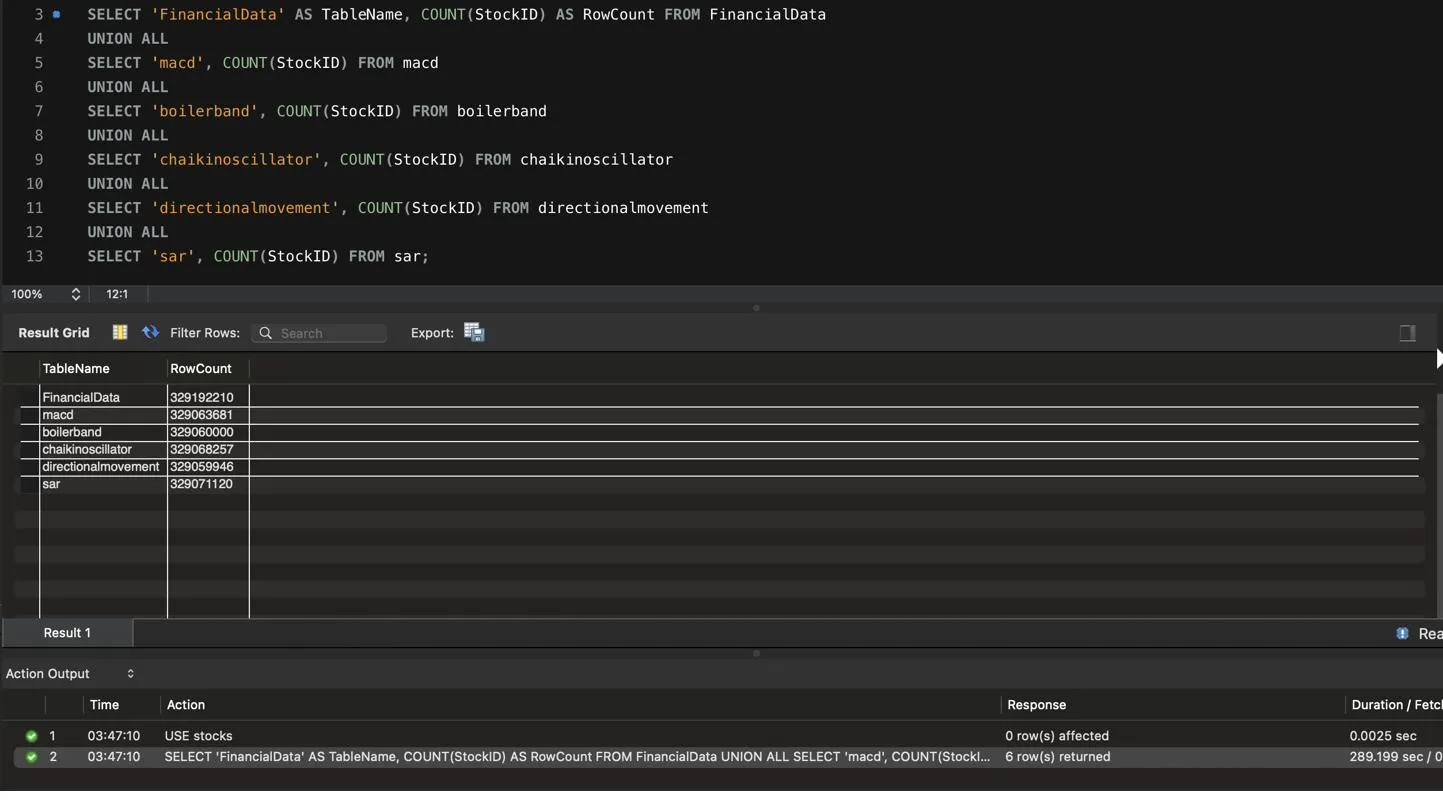
OLTP
InnoDB’s Three Guarantees
Rows store all columns together Fetching one bar for one symbol touches a single spot on disk, which is exactly what ingest wants. An indicator that needs two columns still fetches every column through the buffer pool.
Indexes speed up reads and slow writes Every index is its own B-tree and every write must update all B-trees in the table. B-trees are extremely quick to read. The goal of any index is to speed up reads at the cost of slower writes. Great for selective reads, awful for write heavy ingestion work. Which was my reasoning why my Raw* tables only have a primary key, and why there’s heavy indexing and partitioning on the tables that receive the Raw*’s work.
Undo log allows concurrent reads and writes When a row is updated or deleted, the old value is stored in something called an undo log. If a session reads the table during the write, the old value comes from the undo log. Inserts get a smaller undo log too, the table and the primary key being inserted are stored, so InnoDB knows what to revert if the insert doesn’t commit. On commit an insert’s undo log is purged immediately. An update or delete’s undo log joins a global list called the history list, which is what lets sessions read older versions of changed data. For update and delete heavy databases the history list grows quickly, which would be a nightmare to deal with. Luckily someone smarter than me built the solution and you guessed right, it’s built right into InnoDB. InnoDB flags undo logs to be purged once every session that started before or during the commit has finished. This system is called Multi-Version Concurrency Control, MVCC for short. After all the technical jargon, the English translation is the MVCC allows inserts and updates to happen without blocking reads.
Without knowing, I designed my InnoDB database using an OLAP design fundamental. financialdata held the datetime, open, high, low, and close. It was originally the only table that held datetime. Any technical indicator I wanted to query required a join on the financialdata table to know the date the indicator’s row was calculated for. It was one of my worst data designs. A design I realized wouldn’t work only after the database had over 100GBs of data. Fixing this was brutal.
CREATE TABLE `FinancialData` (
`FinancialDataID` int NOT NULL AUTO_INCREMENT,
`StockID` int NOT NULL,
`StockDate` datetime DEFAULT NULL,
`Open` decimal(20,5) DEFAULT NULL,
`Low` decimal(20,5) DEFAULT NULL,
`High` decimal(20,5) DEFAULT NULL,
`Close` decimal(20,5) DEFAULT NULL,
`Volume` decimal(20,5) DEFAULT NULL,
`EMA` decimal(20,5) DEFAULT NULL,
`VWAP` decimal(20,5) DEFAULT NULL,
`RateOfChange` decimal(20,5) DEFAULT NULL,
`OnBalanceVolume` decimal(20,5) DEFAULT NULL,
PRIMARY KEY (`FinancialDataID`,`StockID`),
UNIQUE KEY `StockID_Date_Idx` (`StockID`,`StockDate`),
KEY `idx3` (`StockID`,`FinancialDataID`,`StockDate`,`Close`)
) ENGINE=InnoDB AUTO_INCREMENT=320075156 DEFAULT CHARSET=utf8mb4 COLLATE=utf8mb4_0900_ai_ci
/*!50100 PARTITION BY HASH (`StockID`)
PARTITIONS 100 */;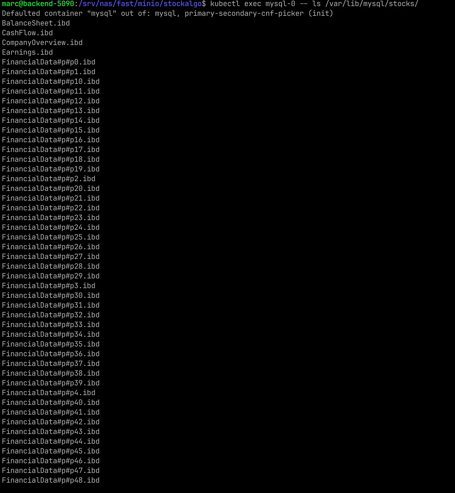 Here’s a picture of the files responsible for my
 financialdata table partition. Each .ibd is an InnoDB tablespace file with roughly 1/100th of the table’s data. The files range: FinancialData#p#p0.ibd - FinancialData#p#p99.ibd.
To be fair, the idea behind the design was sound. financialdata has datetime, open, close, low, high, and StockID, along with quite a few other columns, as you can see from the schema above. When I started this database, I thought I would need these columns for every query. When I started this database, I didn’t even know the most important price is the closing price. Let’s just say I have come a long way, I even read the Wall Street Journal now, and I think we all know what that means. Anyhow, this design meant all of my indicator tables had FinancialDataID and StockID in them, which served as efficient columns to join on. The idea of using financialdata as my base table and “picking” which columns I wanted based on the indicators I was working with sounds pretty darn similar to querying only the columns I want and ignoring the other columns in a table.
When I finally bit the bullet and added StockDate to my indicator tables, I used ole reliable, a stored procedure ran by several different scheduled events. Each scheduled event ran the stored procedure on a separate table, so locking wasn’t an issue, waiting was.
CREATE TEMPORARY TABLE IF NOT EXISTS t
    (StockDate DATETIME, FinancialDataID INT PRIMARY KEY);

INSERT INTO t(StockDate, FinancialDataID)
SELECT StockDate, FinancialDataID FROM FinancialData WHERE StockID = iStockID;

UPDATE sar sr INNER JOIN t on sr.FinancialDataID = t.FinancialDataID SET sr.StockDate = t.StockDate;
UPDATE macd md INNER JOIN t on md.FinancialDataID = t.FinancialDataID SET md.StockDate = t.StockDate;
UPDATE directionalmovement dm INNER JOIN t on dm.FinancialDataID = t.FinancialDataID SET dm.StockDate = t.StockDate;
UPDATE boilerband bb INNER JOIN t on bb.FinancialDataID = t.FinancialDataID SET bb.StockDate = t.StockDate;
UPDATE chaikinoscillator co INNER JOIN t on co.FinancialDataID = t.FinancialDataID SET co.StockDate = t.StockDate;

DROP TEMPORARY TABLE IF EXISTS t;
Each scheduled event ran a single one of these updates, with the other updates commented out.
5 years into v1, I realized my analytical work used 2 or 3 columns per table, while I was forced to read every column. Since optimizing for the analytical work could theoretically give me an edge in the market, I decided to optimize towards it. After doing some research, I came to the conclusion the engine choice was wrong.
OLAP
If you thought the InnoDB section was technical, oh buddy, are you in for a rude awakening.
Version 2’s analytical tables are Iceberg on MinIO, Parquet files behind a Polaris catalog, with Spark handling the reads. The entire partitioning story is one clause of DDL, pulled from here:
CREATE TABLE IF NOT EXISTS raw_bars (`symbol` string, `time_stamp` timestamp, `open` double,
    `high` double, `low` double, `close` double, `volume` bigint, `vwap` double,
    `trade_count` bigint, `is_valid` boolean)
USING iceberg PARTITIONED BY (bucket(16,`symbol`));
One of the luxuries of working with Iceberg is it computes and stores any partition in the metadata. Which means if I want to add a column to the partition I pay the price during reads. Iceberg’s pruning must walk through my previous partitioned data files while walking through the newly partitioned data files. The data is grouped by partition version, pruned independently per version, and the prunes are merged afterwards, all of which happens during split planning. It took several days to a week to partition a table in v1, I had plenty of coffee breaks working with v1, and if I wanted to change a partition, I’d have to re-partition the entire table again, which is why I chose a larger than normal hash of 100. ~13,000 StockIDs split into groups of 130 StockIDs meant it would take YEARS before I had to repartition.
The Read Path
My lakehouse’s query optimizer took me about a month to understand, because it’s a relatively complex topic, plus, it was one of the few ideas I couldn’t relate to my OLTP background. I’m spoiling some of the technical magic, but I struggled to understand the difference between a manifest and a data file. In the scheme of things, these two definitions are on the simpler side, but I couldn’t grasp that grouping of data happened on multiple different layers. Understanding manifests and data files was my ah ha moment. Getting back to the regularly scheduled program, the lakehouse is composed of three pieces, Apache Polaris, MinIO, and Apache Iceberg.
Polaris serves as my catalog, which for me, is a Postgres database and an API to read and write to it. In terms of query optimization, the Postgres database’s main responsibility is to store a pointer to a metadata.json file per Iceberg table. Every query starts by asking for that pointer, and every commit ends by updating it. Polaris only accepts one update at a time, which is what keeps table updates atomic, and what happens when two writers show up at once is covered in the commit path. Obviously this is my favorite piece of the lake house since it has an OLTP database.
MinIO is the physical storage of my lakehouse. The only reason I use MinIO is because I’m hosting my lakehouse in my homelab. The main purpose of MinIO is to store the parquet data files, the manifests and manifest lists, and the metadata.json files. Using MinIO means the file structure is identical to an S3 Bucket. That’s all MinIO is responsible for, replacing the real thing with a homemade one.
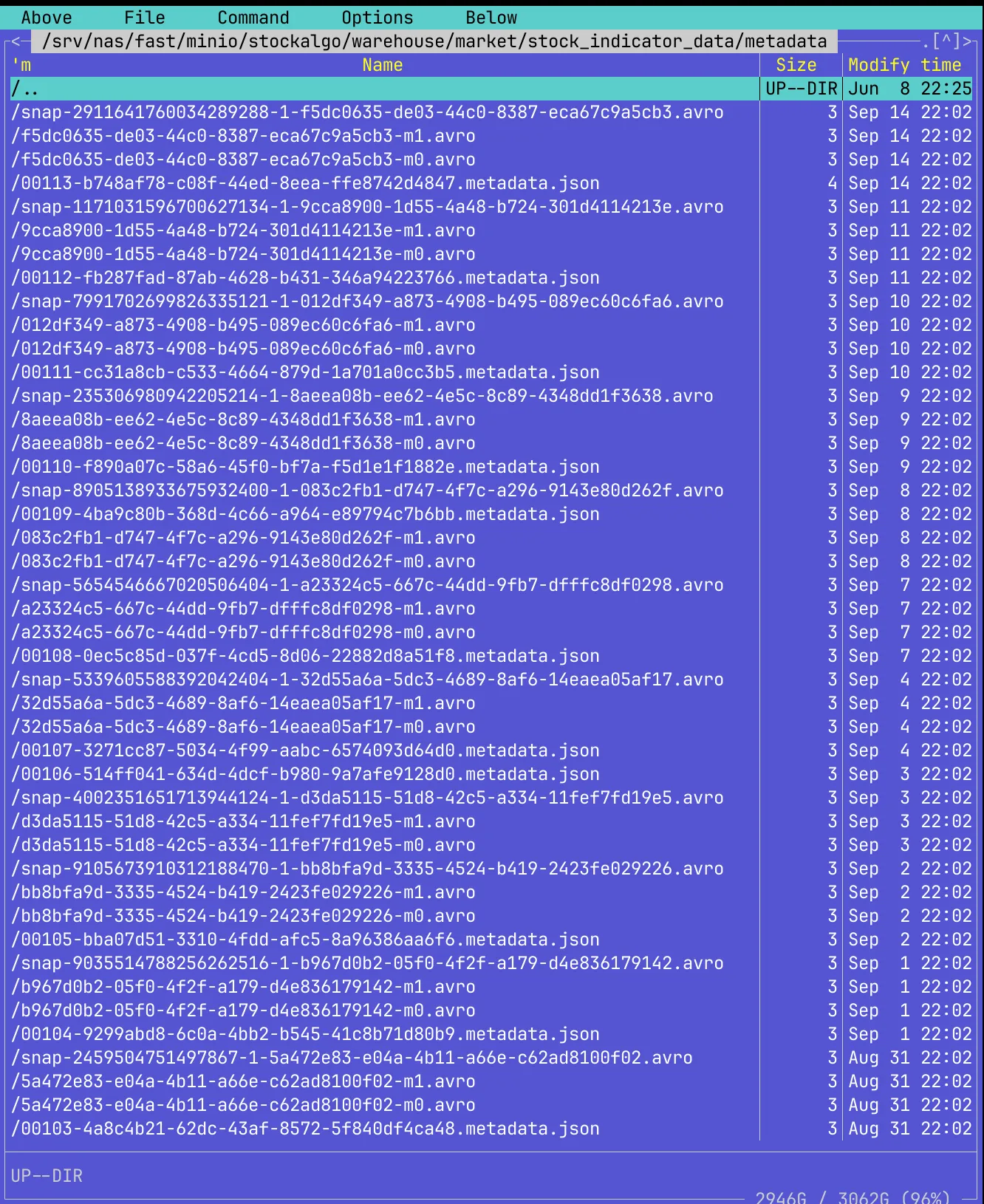 Actual files written for my September commits around 22:02:
 metadata.json = table’s new updated version, snap-*.avro = manifest list, and m0.avro + m1.avro = manifests. Since the market’s closed on Saturday and Sunday the MERGE is empty, so these files don’t exist.
Iceberg is the brains. Polaris and MinIO serve very specific reasons. Iceberg does the rest. Iceberg gives us two layers of query optimization and we get an additional layer of optimization at the data file level. I like to think of the optimization layers as those Russian nesting dolls, we start at the smallest doll and put each doll inside the next smallest doll, building a summary of each layer starting from the data files and ending at the metadata.json files.
The smallest doll is newly written data files. Data files are exactly what they sound like, data in the table written as a file called a parquet file. A parquet file is optimized for columnar systems and lets us pick the column to read instead of always having to read every column. The reason the data files are the smallest doll is because every parquet file has different groups of rows and a summary per grouped rows, specifically min/max and number of nulls per column. By default, the grouped rows, or Row Groups, are batched by the order they arrive. You can define how rows are grouped by using WRITE ORDERED BY. I haven’t used WRITE ORDERED BY in my lakehouse, because I was happy my lakehouse worked and haven’t gone back to add WRITE ORDERED BY symbol, time_stamp DESC. Notice how it’s the same combo my first version used as a unique key.
The next doll we look at is a larger version of the doll we came from. The data files are grouped by something called a Manifest. Just like the Row Groups, a Manifest tracks min/max and null counts per column, and it also tracks each data file’s partition value, file size, and location. The same idea as a Row Group, with a larger summary. Manifests are also responsible for tracking something called Delete Files. Delete Files are exactly what they sound like, they track rows that have been deleted or updated. Manifests link Delete Files to the Data Files, which lets Iceberg remove any rows in the Delete File before giving the query’s results. If Delete Files exist for a table, the merging of the Data Files and the Delete Files happens every read. This is what’s called merge on read. Even though computing on every read instead of computing on a single write seems useless, there’s one very popular purpose, Streaming. It’s a lot faster to jot down what changed and figure it out later instead of making the change.
The largest nested doll is the Manifest list. Exactly like the step before, a Manifest List is a summary from one step above Manifests. The Manifest list gives us the min/max calculated partition value per Manifest, and the partition version each Manifest was written under. Keeping track of the partition version makes the split planning from earlier possible. One Manifest list belongs to one snapshot, and the snapshot stores a pointer to its linked Manifest list file. Both the snapshotID and the Manifest List pointer sit in the metadata.json file. The table’s metadata.json file also tells us the history of the table with snapshotIDs, the Manifest lists that belong to the snapshotIDs, as well as actual metadata about the table telling us about each column. I promise I’m not sponsored (yet), but man is Netflix good at making software.
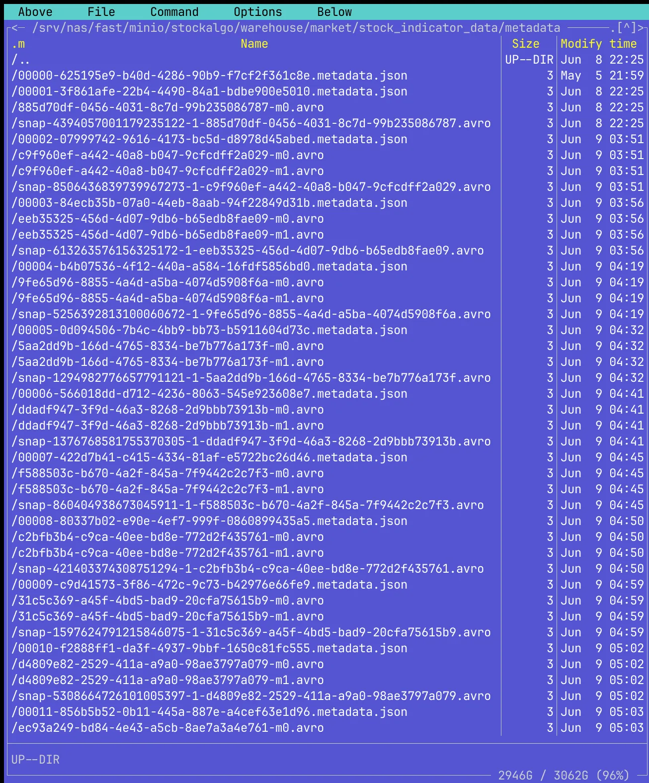 I present to you, the evolution of my lakehouse, on May 5th there were tables! The 0000 indicate this table was the first to migrate into its new home, it was alone without data to accompany it. Skipping forward to June 8th, we see the descendant of the 0000 table, 0001 and it’s accompanied by two avro files,
 *-m0.avro serves as the manifest, while snap-*.avro serves as the manifest list. We can also see the lovely lineage of this lakehouse by following the 000**.metadata.json files. Yeah, I’ve officially lost it…
Instead of chasing how my lakehouse optimizes queries, I’ll walk through what happens for an executor that’s ready to write. A MERGE has to find its matched rows, and the files they live in, before it can rewrite them, so a write starts as a read. The executor starts by asking Polaris for the table’s pointer to the current metadata file. The metadata file names the current snapshot. The snapshot points at its manifest list, and the planner computes my symbol’s bucket and only enters the bucket the symbol belongs in. We check only the Manifests whose partition range contains our calculated symbol. The data files that survived the previous prune check every row group’s statistics to prune any row groups we do not need to check, and we decode the data files of the row groups that are still alive. Three data filtering layers at significantly different levels of the lakehouse. This is the general model behind most columnar warehouses and lakehouses. Snowflake, BigQuery, and Delta Lake run some concoction of it. The high level path is statistics stamped at write time, pruned before any data is read, and columnar decodes, the main difference is the names between vendors. Learning it once meant learning most of them.
My indicator table has 36 columns. When an indicator requires close and volume, I can finally say those two columns are read, while the other 34 stay on disk where they belong. It only took me about 8,000 words and 9 months.
The Commit Path
Data files are immutable. A write makes new files. My ingest lands through a MERGE, pulled from here:
MERGE INTO stockalgo.market.raw_bars AS rb
USING new_raw_bars AS nrb ON rb.symbol = nrb.symbol AND rb.time_stamp = nrb.time_stamp
WHEN MATCHED THEN UPDATE SET rb.time_stamp = nrb.time_stamp, rb.open = nrb.open, rb.close = nrb.close,
rb.high = nrb.high, rb.low = nrb.low, rb.volume= nrb.volume, rb.vwap=nrb.vwap, rb.trade_count = nrb.trade_count,
rb.is_valid = nrb.is_valid
WHEN NOT MATCHED THEN INSERT (symbol, time_stamp, open, close, high, low, volume, vwap, trade_count, is_valid)
VALUES(nrb.symbol, nrb.time_stamp, nrb.open, nrb.close, nrb.high, nrb.low, nrb.volume, nrb.vwap, nrb.trade_count, nrb.is_valid);
Matched rows get their files rewritten as new files, otherwise known as copy on write, the arch enemy of merge on read. If there are unmatched rows, they become appends.
The writer builds new manifests describing the new files, a new manifest list for the new snapshot, and a new metadata file with the snapshot appended to the table’s history. Then it asks Polaris to swap the table’s pointer from the old metadata file to the new one. That swap is atomic, and it is the entire commit. Two writers racing produce two potential metadata files, and the quicker writer checks the table’s current version matches the version it read from, then wins the swap. The slower writer sees the mismatch and checks if the data files that changed in the new table version are the same data files it worked on. If the data files are different, the slower writer reapplies its changes on top of the new current snapshot and attempts the swap again. If the data files are the same, it fails and tries again depending on retry logic. My v1 advisory locks solved the same race the opposite way, the second writer waited its turn instead of losing and retrying.
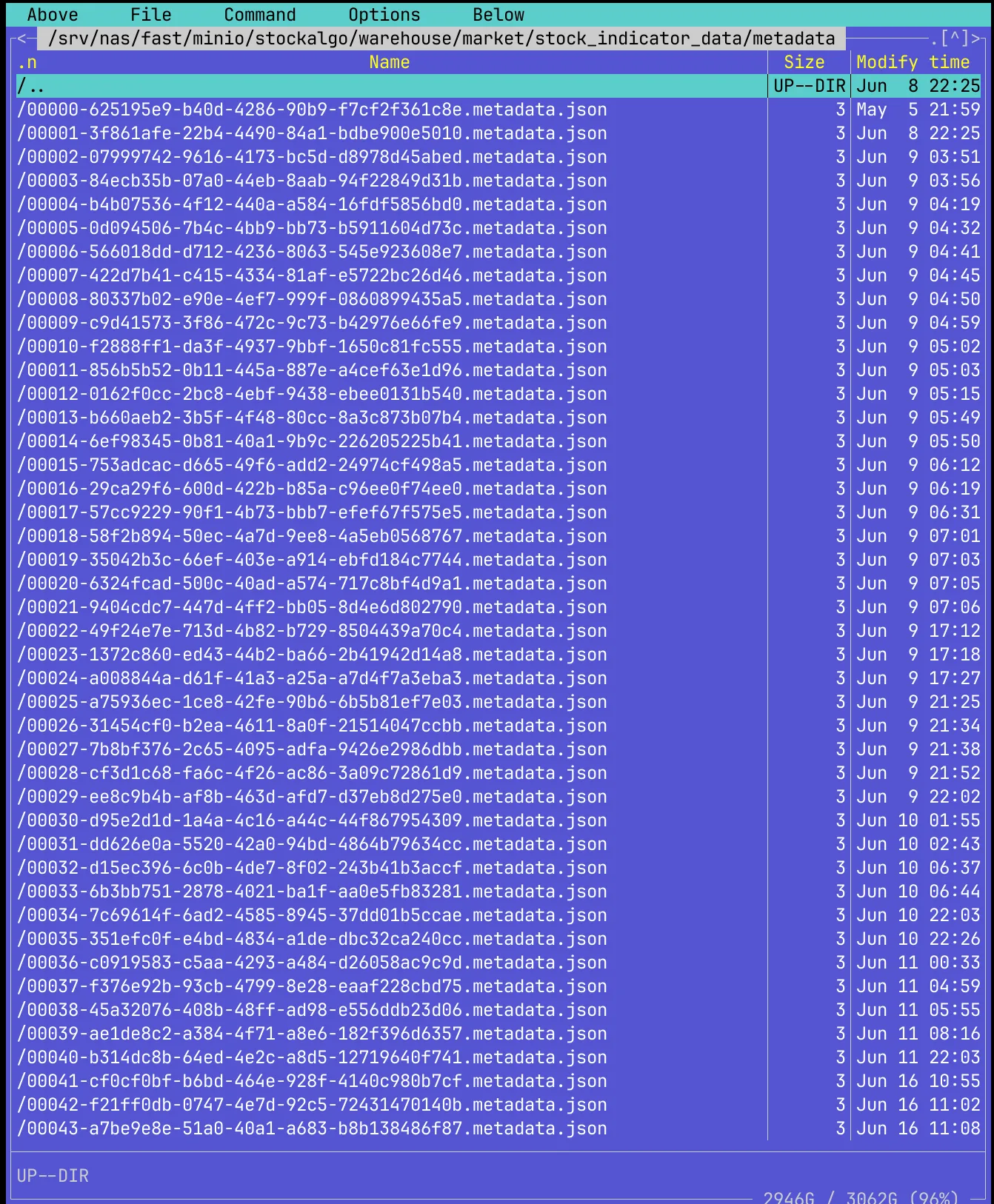 Here we have the rare sighting of 44 retired
 metadata.json files. Believe it or not, but Postgres probably pointed at every single one of these files when they were brand spanking new. Now they serve as a reminder for me to setup automatic deletion of old metadata.json. Let’s be honest, they’re part of the lakehouse now, it would be rude to delete them.
Reads aren’t forced to wait either. A reader holds the snapshot it started with and immutable files can’t change underneath it. InnoDB’s undo log from earlier exists for this exact guarantee. The engine saves the old row version so readers can keep working during a write, and Iceberg skips the saving because the old version is the old file.
A write to my lakehouse that dies midway leaves orphaned data files and no snapshot. No reader ever saw it, and the retry is safe because the MERGE keys make it idempotent. In v1 I used temp tables, anti joins, and deletes after successful commits. In v2 I used MERGE instead of INSERT.
The Comparison
Both engines, same questions:
| Question | InnoDB (v1) | Iceberg + Spark + Polaris (v2) |
|---|---|---|
| What makes a read fast | Secondary B-tree indexes, paid on every write | Metadata at write time, three levels of pruning |
| What a write costs | Row updated in place plus every index | New immutable files plus one snapshot commit |
| Cost of changing the partitioning | A full table rebuild, days to a week | A metadata change, split planning covers old files |
| How a scan reads columns | Full rows through the buffer pool | Only the columns the query names |
| Concurrent writers | Advisory locks I managed | Optimistic pointer swap, loser retries |
| What a reader sees | MVCC row versions | One immutable snapshot |
| A write that dies midway | Temp tables, anti joins, deletes after commit | Orphaned files, no snapshot, retry is idempotent |
| Row count | Index scan across every row | Snapshot summary, metadata read |
| The maintenance bill | Index and partition upkeep | Compaction and snapshot expiration |
The Rest of The Story
The coordination half of v1, the scheduler, the worker pool, and the staging pipeline, is the airflow post. The Spark side of v2, how 13 shuffles became one Exchange, is coming soon to a theater near you. The replication setup MySQL runs on today is the StatefulSet post. The schema and all 41 stored procedures are in the repo’s legacy directory if you want to see what analytics on an OLTP engine looks like up close.